Concepts
Data Model
Metric and Label
Every time series is uniquely identified by its metric name and optional key-value pairs called labels.
The metric name specifies the general feature of a system that is measured (e.g. http_requests_total - the total number of HTTP requests received). It may contain ASCII letters and digits, as well as underscores and colons. It must match the regex [a-zA-Z_:][a-zA-Z0-9_:]*.
Note: The colons are reserved for user defined recording rules. They should not be used by exporters or direct instrumentation.
Labels enable Prometheus’s dimensional data model: any given combination of labels for the same metric name identifies a particular dimensional instantiation of that metric (for example: all HTTP requests that used the method POST to the /api/tracks handler). The query language allows filtering and aggregation based on these dimensions. Changing any label value, including adding or removing a label, will create a new time series.
Label names may contain ASCII letters, numbers, as well as underscores. They must match the regex [a-zA-Z_][a-zA-Z0-9_]*. Label names beginning with __ are reserved for internal use.
Label values may contain any Unicode characters.
A label with an empty label value is considered equivalent to a label that does not exist.
Job and Instance
In Prometheus terms, an endpoint you can scrape is called an instance, usually corresponding to a single process. A collection of instances with the same purpose, a process replicated for scalability or reliability for example, is called a job.
For example, an API server job with four replicated instances:
- job:
api-server- instance 1:
1.2.3.4:5670 - instance 2:
1.2.3.4:5671 - instance 3:
5.6.7.8:5670 - instance 4:
5.6.7.8:5671
- instance 1:
When Prometheus scrapes a target, it attaches some labels automatically to the scraped time series which serve to identify the scraped target:
job: The configured job name that the target belongs to.instance: The<host>:<port>part of the target’s URL that was scraped.
https://prometheus.io/docs/concepts/jobs_instances/
时间序列(Time Series)
在之前,通过Node Exporter暴露的HTTP服务,Prometheus可以采集到当前主机所有监控指标的样本数据。例如:
# HELP node_cpu Seconds the cpus spent in each mode.
# TYPE node_cpu counter
node_cpu{cpu="cpu0",mode="idle"} 362812.7890625
# HELP node_load1 1m load average.
# TYPE node_load1 gauge
node_load1 3.0703125
其中非#开头的每一行表示当前Node Exporter采集到的一个监控样本:node_cpu和node_load1表明了当前指标的名称、大括号中的标签则反映了当前样本的一些特征和维度、浮点数则是该监控样本的具体值。
样本(Sample)
Prometheus会将所有采集到的样本数据以时间序列(time-series)的方式保存在内存数据库中,并且定时保存到硬盘上。time-series是按照时间戳和值的序列顺序存放的,我们称之为向量(vector). 每条time-series通过指标名称(metrics name)和一组标签集(labelset)命名。如下所示,可以将time-series理解为一个以时间为Y轴的数字矩阵:
  ^
  │   . . . . . . . . . . . . . . . . .   . .   node_cpu{cpu="cpu0",mode="idle"}
  │     . . . . . . . . . . . . . . . . . . .   node_cpu{cpu="cpu0",mode="system"}
  │     . . . . . . . . . .   . . . . . . . .   node_load1{}
  │     . . . . . . . . . . . . . . . .   . .
  v
    <------------------ 时间 ---------------->
在time-series中的每一个点称为一个样本(sample),样本由以下三部分组成:
- 指标(metric):metric name 描述当前样本特征的labelsets;
- 时间戳(timestamp):一个精确到毫秒的时间戳;
- 样本值(value): 一个float64的浮点型数据表示当前样本的值。
<--------------- metric ---------------------><-timestamp -><-value->
http_request_total{status="200", method="GET"}@1434417560938 => 94355
http_request_total{status="200", method="GET"}@1434417561287 => 94334


http_request_total{status="404", method="GET"}@1434417560938 => 38473
http_request_total{status="404", method="GET"}@1434417561287 => 38544


http_request_total{status="200", method="POST"}@1434417560938 => 4748
http_request_total{status="200", method="POST"}@1434417561287 => 4785
Prometheus Metrics Format
https://prometheus.io/docs/instrumenting/exposition_formats/
Metrics Type
在Prometheus的存储实现上所有的监控样本都是以time-series的形式保存在Prometheus内存的TSDB(时序数据库)中,而time-series所对应的监控指标(metric)也是通过labelset进行唯一命名的。
从存储上来讲所有的监控指标metric都是相同的,但是在不同的场景下这些metric又有一些细微的差异。 例如,在Node Exporter返回的样本中指标node_load1反应的是当前系统的负载状态,随着时间的变化这个指标返回的样本数据是在不断变化的。而指标node_cpu所获取到的样本数据却不同,它是一个持续增大的值,因为其反应的是CPU的累积使用时间,从理论上讲只要系统不关机,这个值是会无限变大的。
为了能够帮助用户理解和区分这些不同监控指标之间的差异,Prometheus定义了4种不同的指标类型(metric type):Counter(计数器)、Gauge(仪表盘)、Histogram(直方图)、Summary(摘要)。
在Exporter返回的样本数据中,其注释中也包含了该样本的类型。例如:
# HELP node_cpu Seconds the cpus spent in each mode.
# TYPE node_cpu counter
node_cpu{cpu="cpu0",mode="idle"} 362812.7890625
https://prometheus.io/docs/concepts/metric_types/
Counter - 只增不减的计数器
Counter类型的指标其工作方式和计数器一样,只增不减(除非系统发生重置)。常见的监控指标,如http_requests_total,node_cpu都是Counter类型的监控指标。 一般在定义Counter类型指标的名称时推荐使用_total作为后缀。
Counter是一个简单但有强大的工具,例如我们可以在应用程序中记录某些事件发生的次数,通过以时序的形式存储这些数据,我们可以轻松的了解该事件产生速率的变化。 PromQL内置的聚合操作和函数可以让用户对这些数据进行进一步的分析:
# HELP node_cpu_seconds_total Seconds the cpus spent in each mode.
# TYPE node_cpu_seconds_total counter
node_cpu_seconds_total{cpu="0",mode="idle"} 177396.3
node_cpu_seconds_total{cpu="0",mode="nice"} 0

# From /metrics
# HELP promotion_promhttp_metric_handler_requests_total Total number of scrapes by HTTP status code.
# TYPE promotion_promhttp_metric_handler_requests_total counter
promotion_promhttp_metric_handler_requests_total{code="200",service_name="promotion.logistics"} 9
promotion_promhttp_metric_handler_requests_total{code="500",service_name="promotion.logistics"} 0
promotion_promhttp_metric_handler_requests_total{code="503",service_name="promotion.logistics"} 0
例如,通过 rate() 函数获取HTTP请求量的增长率:
rate(http_requests_total[5m])
查询当前系统中,访问量前10的HTTP地址:
topk(10, http_requests_total)
Gauge - 可增可减的仪表盘
A gauge is a metric that represents a single numerical value that can arbitrarily go up and down.
Gauges are typically used for measured values like temperatures or current memory usage, but also “counts” that can go up and down, like the number of concurrent requests.
与Counter不同,Gauge类型的指标侧重于反应系统的当前状态。因此这类指标的样本数据可增可减。常见指标如:node_memory_MemFree(主机当前空闲的内容大小)、node_memory_MemAvailable(可用内存大小)都是Gauge类型的监控指标。
Example:
# TYPE node_filesystem_free_bytes gauge
node_filesystem_free_bytes{device="/dev/disk1s1",fstype="apfs",mountpoint="/System/Volumes/Data"} 2.1108973568e+11
node_filesystem_free_bytes{device="/dev/disk1s4",fstype="apfs",mountpoint="/private/var/vm"} 4.92446932992e+11
node_filesystem_free_bytes{device="/dev/disk1s5",fstype="apfs",mountpoint="/"} 4.88740073472e+11
node_filesystem_free_bytes{device="map -fstab",fstype="autofs",mountpoint="/System/Volumes/Data/Network/Servers"} 0
node_filesystem_free_bytes{device="map auto_home",fstype="autofs",mountpoint="/System/Volumes/Data/home"} 0
# HELP node_filesystem_readonly Filesystem read-only status.
通过Gauge指标,用户可以直接查看系统的当前状态:
node_memory_MemFree
对于Gauge类型的监控指标,通过PromQL内置函数delta()可以获取样本在一段时间返回内的变化情况。例如,计算CPU温度在两个小时内的差异:
delta(cpu_temp_celsius{host="zeus"}[2h])
还可以使用deriv()计算样本的线性回归模型,甚至是直接使用predict_linear()对数据的变化趋势进行预测。例如,预测系统磁盘空间在4个小时之后的剩余情况:
predict_linear(node_filesystem_free{job="node"}[1h], 4 * 3600)
Histogram/Summary - 分析数据分布情况
除了Counter和Gauge类型的监控指标以外,Prometheus还定义了Histogram和Summary的指标类型。Histogram和Summary主用用于统计和分析样本的分布情况。
在大多数情况下人们都倾向于使用某些量化指标的平均值,例如CPU的平均使用率、页面的平均响应时间。
这种方式的问题很明显,以系统API调用的平均响应时间为例:如果大多数API请求都维持在100ms的响应时间范围内,而个别请求的响应时间需要5s,那么就会导致某些WEB页面的响应时间落到中位数的情况,而这种现象被称为长尾问题(Long-tail Problem)。
为了区分是平均的慢还是长尾的慢,最简单的方式就是按照请求延迟的范围进行分组。例如,统计延迟在0~10ms之间的请求数有多少而10~20ms之间的请求数又有多少。通过这种方式可以快速分析系统慢的原因。Histogram和Summary都是为了能够解决这样问题的存在,通过Histogram和Summary类型的监控指标,我们可以快速了解监控样本的分布情况。
Histogram
A histogram samples observations (usually things like request durations or response sizes) and counts them in configurable buckets. It also provides a sum of all observed values.
A histogram with a base metric name of <basename> exposes multiple time series during a scrape:
- cumulative counters for the observation buckets, exposed as
<basename>_bucket{le="<upper inclusive bound>"} - the total sum of all observed values, exposed as
<basename>_sum - the count of events that have been observed, exposed as
<basename>_count(identical to<basename>_bucket{le="+Inf"}above)
Example
Example 1
在Prometheus Server自身返回的样本数据中,我们还能找到类型为Histogram的监控指标prometheus_tsdb_compaction_chunk_range_bucket。
# HELP prometheus_tsdb_compaction_chunk_range Final time range of chunks on their first compaction
# TYPE prometheus_tsdb_compaction_chunk_range histogram
prometheus_tsdb_compaction_chunk_range_bucket{le="100"} 0
prometheus_tsdb_compaction_chunk_range_bucket{le="400"} 0
prometheus_tsdb_compaction_chunk_range_bucket{le="1600"} 0
prometheus_tsdb_compaction_chunk_range_bucket{le="6400"} 0
prometheus_tsdb_compaction_chunk_range_bucket{le="25600"} 0
prometheus_tsdb_compaction_chunk_range_bucket{le="102400"} 0
prometheus_tsdb_compaction_chunk_range_bucket{le="409600"} 0
prometheus_tsdb_compaction_chunk_range_bucket{le="1.6384e+06"} 260
prometheus_tsdb_compaction_chunk_range_bucket{le="6.5536e+06"} 780
prometheus_tsdb_compaction_chunk_range_bucket{le="2.62144e+07"} 780
prometheus_tsdb_compaction_chunk_range_bucket{le="+Inf"} 780
prometheus_tsdb_compaction_chunk_range_sum 1.1540798e+09
prometheus_tsdb_compaction_chunk_range_count 780
与Summary类型的指标相似之处在于Histogram类型的样本同样会反应当前指标的记录的总数(以_count作为后缀)以及其值的总量(以_sum作为后缀)。不同在于Histogram指标直接反应了在不同区间内样本的个数,区间通过标签len进行定义。
Example 2
# HELP processor_duration_nanoseconds
# TYPE processor_duration_nanoseconds histogram
processor_duration_nanoseconds_bucket{command="cmd1",result_code="0",le="5e+06"} 0
->5000000ns -> 5ms
processor_duration_nanoseconds_bucket{command="cmd1",result_code="0",le="1e+07"} 0
processor_duration_nanoseconds_bucket{command="cmd1",result_code="0",le="2e+07"} 0
processor_duration_nanoseconds_bucket{command="cmd1",result_code="0",le="3e+07"} 0
processor_duration_nanoseconds_bucket{command="cmd1",result_code="0",le="4e+07"} 0
processor_duration_nanoseconds_bucket{command="cmd1",result_code="0",le="5e+07"} 0
processor_duration_nanoseconds_bucket{command="cmd1",result_code="0",le="7e+07"} 0
70,000,000ns -> 70ms
processor_duration_nanoseconds_bucket{command="cmd1",result_code="0",le="1e+08"} 1
100000000ns -> 100ms
processor_duration_nanoseconds_bucket{command="cmd1",result_code="0",le="1.5e+08"} 1
processor_duration_nanoseconds_bucket{command="cmd1",result_code="0",le="2.5e+08"} 1
processor_duration_nanoseconds_bucket{command="cmd1",result_code="0",le="5e+08"} 1
processor_duration_nanoseconds_bucket{command="cmd1",result_code="0",le="1e+09"} 1
processor_duration_nanoseconds_bucket{command="cmd1",result_code="0",le="1.5e+09"} 1
processor_duration_nanoseconds_bucket{command="cmd1",result_code="0",le="2e+09"} 1
processor_duration_nanoseconds_bucket{command="cmd1",result_code="0",le="5e+09"} 1
processor_duration_nanoseconds_bucket{command="cmd1",result_code="0",le="+Inf"} 1
如果一个request的latency为80ms,则 >=70 的所有 bucket都会加1。
Usage
对于Histogram的指标,我们还可以通过 histogram_quantile() 函数计算出其值的分位数。不同在于Histogram通过histogram_quantile函数是在服务器端计算的分位数。 而Sumamry的分位数则是直接在客户端计算完成。因此对于分位数的计算而言,Summary在通过PromQL进行查询时有更好的性能表现,而Histogram则会消耗更多的资源。反之对于客户端而言Histogram消耗的资源更少。在选择这两种方式时用户应该按照自己的实际场景进行选择。
Summary
Similar to a histogram, a summary samples observations (usually things like request durations and response sizes). While it also provides a total count of observations and a sum of all observed values, it calculates configurable quantiles over a sliding time window.
A summary with a base metric name of <basename> exposes multiple time series during a scrape:
- streaming φ-quantiles (0 ≤ φ ≤ 1) of observed events, exposed as
<basename>{quantile="<φ>"} - the total sum of all observed values, exposed as
<basename>_sum - the count of events that have been observed, exposed as
<basename>_count
Example
例如,指标prometheus_tsdb_wal_fsync_duration_seconds的指标类型为Summary。 它记录了Prometheus Server中wal_fsync处理的处理时间,通过访问Prometheus Server的/metrics地址,可以获取到以下监控样本数据:
# HELP prometheus_tsdb_wal_fsync_duration_seconds Duration of WAL fsync.
# TYPE prometheus_tsdb_wal_fsync_duration_seconds summary
prometheus_tsdb_wal_fsync_duration_seconds{quantile="0.5"} 0.012352463
prometheus_tsdb_wal_fsync_duration_seconds{quantile="0.9"} 0.014458005
prometheus_tsdb_wal_fsync_duration_seconds{quantile="0.99"} 0.017316173
prometheus_tsdb_wal_fsync_duration_seconds_sum 2.888716127000002
prometheus_tsdb_wal_fsync_duration_seconds_count 216
从上面的样本中可以得知当前Prometheus Server进行wal_fsync操作的总次数为216次,耗时2.888716127000002s。其中中位数(quantile=0.5)的耗时为0.012352463,9分位数(quantile=0.9)的耗时为0.014458005s。
Difference Between Histogram and Summary
You can use both summaries and histograms to calculate so-called φ-quantiles, where 0 ≤ φ ≤ 1. The φ-quantile is the observation value that ranks at number φ*N among the N observations. Examples for φ-quantiles: The 0.5-quantile is known as the median. The 0.95-quantile is the 95th percentile.
The essential difference between summaries and histograms is that summaries calculate streaming φ-quantiles on the client side and expose them directly, while histograms expose bucketed observation counts and the calculation of quantiles from the buckets of a histogram happens on the server side using the histogram_quantile() function.
The two approaches have a number of different implications:
| Histogram | Summary | |
|---|---|---|
| Required configuration | Pick buckets suitable for the expected range of observed values. | Pick desired φ-quantiles and sliding window. Other φ-quantiles and sliding windows cannot be calculated later. |
| Client performance | Observations are very cheap as they only need to increment counters. | Observations are expensive due to the streaming quantile calculation. |
| Server performance | The server has to calculate quantiles. You can use recording rules should the ad-hoc calculation take too long (e.g. in a large dashboard). | Low server-side cost. |
Number of time series (in addition to the _sum and _count series) |
One time series per configured bucket. | One time series per configured quantile. |
| Quantile error (see below for details) | Error is limited in the dimension of observed values by the width of the relevant bucket. | Error is limited in the dimension of φ by a configurable value. |
| Specification of φ-quantile and sliding time-window | Ad-hoc with Prometheus expressions. | Preconfigured by the client. |
| Aggregation | Ad-hoc with Prometheus expressions. | In general not aggregatable. |
Configuration - prometheus.yml
https://prometheus.io/docs/prometheus/latest/configuration/configuration/
job_name
我们让Prometheus可以从node exporter暴露的服务中获取监控指标数据。
scrape_configs:
  - job_name: 'prometheus'
    static_configs:
      - targets: ['localhost:9090']
  - job_name: 'node'
    static_configs:
      - targets: ['localhost:9100']
当我们需要采集不同的监控指标(例如:主机、MySQL、Nginx)时,我们只需要运行相应的监控采集程序,并且让Prometheus Server知道这些Exporter实例的访问地址。在Prometheus中,每一个暴露监控样本数据的HTTP服务称为一个实例。例如在当前主机上运行的node exporter可以被称为一个实例(Instance)。
而一组用于相同采集目的的实例,或者同一个采集进程的多个副本则通过一个一个任务(Job)进行管理。
当前在每一个Job中主要使用了静态配置(static_configs)的方式定义监控目标。除了静态配置每一个Job的采集Instance地址以外,Prometheus还支持与DNS、Consul、E2C、Kubernetes等进行集成实现自动发现Instance实例,并从这些Instance上获取监控数据。
Recording Rules
Refer to https://swsmile:info/post/prometheus-recording-rule/
Alerting Rules
Alerting rules allow you to define alert conditions based on Prometheus expression language expressions and to send notifications about firing alerts to an external service. Whenever the alert expression results in one or more vector elements at a given point in time, the alert counts as active for these elements’ label sets.
Defining alerting rules
Alerting rules are configured in Prometheus in the same way as recording rules.
An example rules file with an alert would be:
groups:
- name: example
  rules:
  - alert: HighRequestLatency
    expr: job:request_latency_seconds:mean5m{job="myjob"} > 0.5
    for: 10m
    labels:
      severity: page
    annotations:
      summary: High request latency
The optional for clause causes Prometheus to wait for a certain duration between first encountering a new expression output vector element and counting an alert as firing for this element. In this case, Prometheus will check that the alert continues to be active during each evaluation for 10 minutes before firing the alert. Elements that are active, but not firing yet, are in the pending state.
The labels clause allows specifying a set of additional labels to be attached to the alert. Any existing conflicting labels will be overwritten. The label values can be templated.
The annotations clause specifies a set of informational labels that can be used to store longer additional information such as alert descriptions or runbook links. The annotation values can be templated.
https://prometheus.io/docs/prometheus/latest/configuration/alerting_rules/
Alertmanager
The Alertmanager handles alerts sent by client applications such as the Prometheus server. It takes care of deduplicating, grouping, and routing them to the correct receiver integration such as email, PagerDuty, or OpsGenie. It also takes care of silencing and inhibition of alerts.
The following describes the core concepts the Alertmanager implements. Consult the configuration documentation to learn how to use them in more detail.
Grouping Grouping categorizes alerts of similar nature into a single notification. This is especially useful during larger outages when many systems fail at once and hundreds to thousands of alerts may be firing simultaneously.
Example: Dozens or hundreds of instances of a service are running in your cluster when a network partition occurs. Half of your service instances can no longer reach the database. Alerting rules in Prometheus were configured to send an alert for each service instance if it cannot communicate with the database. As a result hundreds of alerts are sent to Alertmanager.
As a user, one only wants to get a single page while still being able to see exactly which service instances were affected. Thus one can configure Alertmanager to group alerts by their cluster and alertname so it sends a single compact notification.
Grouping of alerts, timing for the grouped notifications, and the receivers of those notifications are configured by a routing tree in the configuration file.
Miscellaneous
拉数据问题
下面设置指定Grafana 多久去 Prometheus Server 拉一次数据:
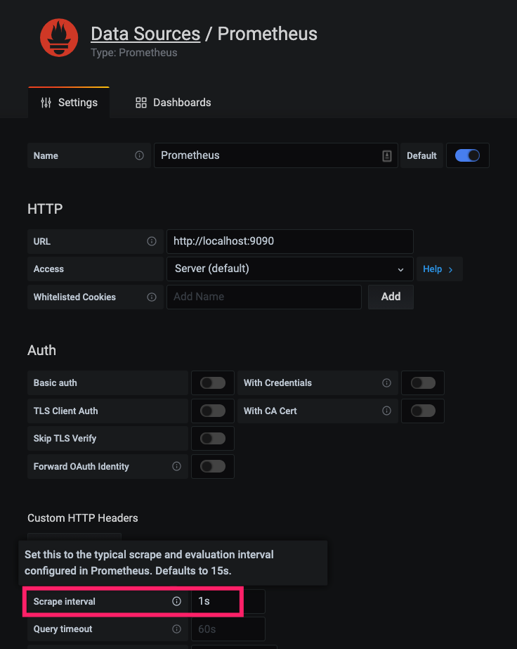
下面设置指定 Grafana 多久刷新一次 Dashboard,但这并不意味着在这段时间Grafna没有去Prometheus Server 拉数据(多久拉一次数据取决于 Scrape interval 的设置)。
如果在这段时间中,去拉了数据(比如Scrape interval 设置为1s,而Refresh dashboard设置为5s,则每5s刷新一次grafana界面,数据采样精度且显示精度为1s)。

结论
- Scrape interval 的设置需要大于等于
prometheus.yml中的global.scrape_interval的设置,等于通常为最佳实践(且设置为15s)- 如果 Scrape interval 的设置需要小于
prometheus.yml中的global.scrape_interval,这会增加Prometheus Server 的压力,但却没有任何意义(不会提高显示精度),因为Prometheus Server 去数据源拉数据的时间间隔大于Grafana去Prometheus Server 拉数据的时间间隔
- 如果 Scrape interval 的设置需要小于
下面设置表示 Prometheus Server 多久去 target server pull 一次数据(即通过访问 /metrics)
# prometheus.yml
global:
  scrape_interval:     15s
科学计数法
8.214304e+06表示 8.214304 * $10^6$。
Reference
- https://prometheus.io/docs/prometheus/latest/querying/basics/
- https://github.com/prometheus/prometheus
- https://prometheus.io/docs/prometheus/
- https://yunlzheng.gitbook.io/prometheus-book/parti-prometheus-ji-chu/promql/prometheus-query-language
- https://en.wikipedia.org/wiki/Time_series
- https://blog.csdn.net/palet/article/details/82763695
- https://prometheus.io/docs/prometheus/latest/querying/functions/
- https://www.metricfire.com/blog/understanding-the-prometheus-rate-function/
- https://medium.com/javarevisited/create-recording-rules-in-prometheus-8a6a1c0b9e11