rate() - per-second average rate
rate(v range-vector) calculates the per-second average rate of increase of the time series in the range vector(每秒增量的平均值).
Breaks in monotonicity (such as counter resets due to target restarts) are automatically adjusted for.
- Also, the calculation extrapolates to the ends of the time range, allowing for missed scrapes or imperfect alignment of scrape cycles with the range’s time period.
The following example expression returns the per-second rate of HTTP requests as measured over the last 5 minutes, per time series in the range vector:
rate(http_requests_total{job="api-server"}[5m])
rate should only be used with counters. It is best suited for alerting, and for graphing of slow-moving counters.
Note that when combining rate() with an aggregation operator (e.g. sum()) or a function aggregating over time (any function ending in _over_time), always take a rate() first, then
Ref to https://prometheus.io/docs/prometheus/latest/querying/functions/#rate
Experiment
https://blog.doit-intl.com/making-peace-with-prometheus-rate-43a3ea75c4cf
Example
Return the 5-minute rate of the http_requests_total metric for the past 30 minutes, with a resolution of 1 minute.
rate(http_requests_total[5m])[30m:1m]
irate() - last two data points
irate(v range-vector) calculates the per-second instant rate of increase of the time series in the range vector. This is based on the last two data points(取最近两个数据点来算速率). Breaks in monotonicity (such as counter resets due to target restarts) are automatically adjusted for.
The following example expression returns the per-second rate of HTTP requests looking up to 5 minutes back for the two most recent data points, per time series in the range vector:
irate(http_requests_total{job="api-server"}[5m])
irate should only be used when graphing volatile, fast-moving counters. Use rate for alerts and slow-moving counters, as brief changes in the rate can reset the FOR clause and graphs consisting entirely of rare spikes are hard to read.
Note that when combining irate() with an aggregation operator (e.g. sum()) or a function aggregating over time (any function ending in _over_time), always take a irate() first, then aggregate. Otherwise irate() cannot detect counter resets when your target restarts.
Experiment
Look at the following picture for hypothetical requests_total counter:
v  20     50     100     200     201      230
----x-+----x------x-------x-------x--+-----x-----
t  10 |   20     30      40      50  |     60
      |   <--     range=40s      --> |
                                     ^
                                     t
It contains values [20,50,100,200,201,230] with timestamps [10,20,30,40,50,60]. Let’s calculate irate(requests_total[40s]) at the point t. It is calculated as dv/dt for the last two points before t according to the documentation:
(201–200) / (50–40) = 0.1 rps
The 40s range ending at t contains other per-second rates:
(100–50) / (30–20) = 5 rps(200–100) / (40–30) = 10 rps
These rates are much larger than the captured rate at t. irate captures only 0.1 rps while skipping 5 and 10 rps. Obviously irate doesn’t capture spikes.
Ref
Discussion
rate() vs increase()
如下图所示,样本增长率反映出了样本变化的剧烈程度:
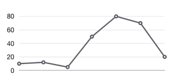
通过增长率表示样本的变化情况
increase(v range-vector)函数是PromQL中提供的众多内置函数之一。其中参数v是一个区间向量,increase函数获取区间向量中的第一个后最后一个样本并返回其增长量。因此,可以通过以下表达式Counter类型指标的增长率:
increase(node_cpu[2m]) / 120
这里通过node_cpu[2m]获取时间序列最近两分钟的所有样本,increase计算出最近两分钟的增长量,最后除以时间120秒得到node_cpu样本在最近两分钟的平均增长率。并且这个值也近似于主机节点最近两分钟内的平均CPU使用率。
除了使用increase函数以外,PromQL中还直接内置了rate(v range-vector) 函数,rate函数可以直接计算区间向量v在时间窗口内平均增长速率。因此,通过以下表达式可以得到与increase函数相同的结果:
rate(node_cpu[2m])
需要注意的是使用rate或者increase函数去计算样本的平均增长速率,容易陷入“长尾问题”当中,其无法反应在时间窗口内样本数据的突发变化。 例如,对于主机而言在2分钟的时间窗口内,可能在某一个由于访问量或者其它问题导致CPU占用100%的情况,但是通过计算在时间窗口内的平均增长率却无法反应出该问题。
为了解决该问题,PromQL提供了另外一个灵敏度更高的函数 irate(v range-vector)。irate同样用于计算区间向量的计算率,但是其反应出的是瞬时增长率。irate函数是通过区间向量中最后两个样本数据来计算区间向量的增长速率。这种方式可以避免在时间窗口范围内的“长尾问题”,并且体现出更好的灵敏度,通过irate函数绘制的图标能够更好的反应样本数据的瞬时变化状态。
irate(node_cpu[2m])
irate函数相比于rate函数提供了更高的灵敏度,不过当需要分析长期趋势或者在告警规则中,irate的这种灵敏度反而容易造成干扰。因此在长期趋势分析或者告警中更推荐使用rate函数。
rate() 与 irate() 的区别
irate和rate都会用于计算某个指标在一定时间间隔内的变化速率。但是它们的计算方法有所不同:irate只取在指定时间范围内的第一个和最后一个数据点来算速率(这意味着如果中间还有采样点,这些点会被直接忽略),而rate会取指定时间范围内的每一个数据点,并算出一组速率,然后取平均值作为结果。
所以官网文档说:irate适合快速变化的计数器(counter),而rate适合缓慢变化的计数器(counter)。
比如CPU usage,我们认为是缓慢变化的计数器(counter)。
实验
我们来看看CPU的idle 百分百:
# irate
irate(node_cpu_seconds_total{cpu="0",mode="idle"}[10m])
# rate
rate(node_cpu_seconds_total{cpu="0",mode="idle"}[10m])
可以看到,irate的曲线比较曲折,而rate的曲线相对平缓:
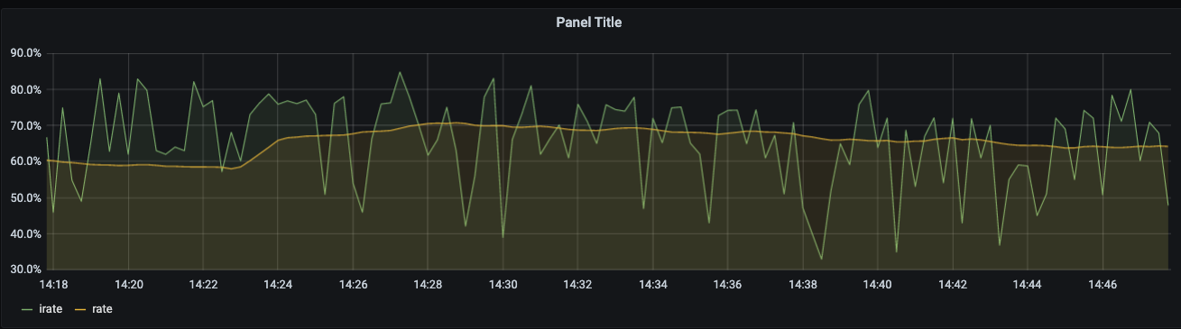
这其实是因为:
-
rate()会取每秒增量的平均值,取平均值意味着当CPU 的idle 在采样时间点陡增时(我们假设这个陡增只是在一个微小的瞬间陡增了,而在此之前和之后的值几乎一致),在图中并不会很明显(因为被平均掉了) -
irate()会取最近两个数据点来算速率,这意味着如果当CPU 的idle 在采样时间点陡增时,
如何设置 time range
What time range should we choose? There is no silver bullet here: at the very minimum it should be two times the scrape interval. However, in this case the result will be very “sharp”: all of the changes in the value would reflect in the results of the function faster than any other time range. Thereafter, the result would become 0 again swiftly. Increasing the time range would achieve the opposite - the resulting line (if you plotted the results) would become “smoother” and it would be harder to spot the spikes. Thus, the recommendation is to put the time range into a different variable (let’s say 1m, 5m, 15m, 2h) in Grafana, then you are able to choose whichever value fits your case the best at the time when you are trying to spot something - such as a spike or a trend.
Extrapolation: what rate() does when missing information
Last but not least, it’s important to understand that rate() performs extrapolation. Knowing this will save you from headaches in the long-term. Sometimes when rate() is executed in a point in time, there might be some data missing if some of the scrapes had failed. What’s more, the scrape interval due to added randomness might not align perfectly with the range vector, even if it is a multiple of the range vector’s time range.
In such a case, rate() calculates the rate with the data that it has and then, if there is any information missing, extrapolates the beginning or the end of the selected window using either the first or last two data points. This means that you might get uneven results even if all of the data points are integers, so this function is suited only for spotting trends, spikes, and for alerting if something happens.
histogram_quantile()
histogram_quantile(φ scalar, b instant-vector) calculates the φ-quantile (0 ≤ φ ≤ 1) from the buckets b of a histogram.
The samples in b are the counts of observations in each bucket. Each sample must have a label le where the label value denotes the inclusive upper bound of the bucket. (Samples without such a label are silently ignored.) The histogram metric type automatically provides time series with the _bucket suffix and the appropriate labels.
Use the rate() function to specify the time window for the quantile calculation.
Example: A histogram metric is called http_request_duration_seconds. To calculate the 90th percentile of request durations over the last 10m, use the following expression:
histogram_quantile(0.9, rate(http_request_duration_seconds_bucket[10m]))
The quantile is calculated for each label combination in http_request_duration_seconds. To aggregate, use the sum() aggregator around the rate() function. Since the le label is required by histogram_quantile(), it has to be included in the by clause. The following expression aggregates the 90th percentile by job:
histogram_quantile(0.9, sum by (job, le) (rate(http_request_duration_seconds_bucket[10m])))
To aggregate everything, specify only the le label:
histogram_quantile(0.9, sum by (le) (rate(http_request_duration_seconds_bucket[10m])))
The histogram_quantile() function interpolates quantile values by assuming a linear distribution within a bucket. The highest bucket must have an upper bound of +Inf. (Otherwise, NaN is returned.) If a quantile is located in the highest bucket, the upper bound of the second highest bucket is returned. A lower limit of the lowest bucket is assumed to be 0 if the upper bound of that bucket is greater than 0. In that case, the usual linear interpolation is applied within that bucket. Otherwise, the upper bound of the lowest bucket is returned for quantiles located in the lowest bucket.
If b has 0 observations, NaN is returned. If b contains fewer than two buckets, NaN is returned. For φ < 0, -Inf is returned. For φ > 1, +Inf is returned.
<aggregation>_over_time()
The following functions allow aggregating each series of a given range vector over time and return an instant vector with per-series aggregation results:
avg_over_time(range-vector): the average value of all points in the specified interval.min_over_time(range-vector): the minimum value of all points in the specified interval.max_over_time(range-vector): the maximum value of all points in the specified interval.sum_over_time(range-vector): the sum of all values in the specified interval.count_over_time(range-vector): the count of all values in the specified interval.quantile_over_time(scalar, range-vector): the φ-quantile (0 ≤ φ ≤ 1) of the values in the specified interval.stddev_over_time(range-vector): the population standard deviation of the values in the specified interval.stdvar_over_time(range-vector): the population standard variance of the values in the specified interval.
Note that all values in the specified interval have the same weight in the aggregation even if the values are not equally spaced throughout the interval.
delta()
delta(v range-vector) calculates the difference between the first and last value of each time series element in a range vector v, returning an instant vector with the given deltas and equivalent labels. The delta is extrapolated to cover the full time range as specified in the range vector selector, so that it is possible to get a non-integer result even if the sample values are all integers.
The following example expression returns the difference in CPU temperature between now and 2 hours ago:
delta(cpu_temp_celsius{host="zeus"}[2h])
delta should only be used with gauges.
increase()
Reference
- https://prometheus.io/docs/prometheus/latest/querying/functions/
- https://www.robustperception.io/how-does-a-prometheus-counter-work
- https://www.robustperception.io/irate-graphs-are-better-graphs
- https://valyala.medium.com/why-irate-from-prometheus-doesnt-capture-spikes-45f9896d7832