Pre-envolution
Consider the world’s simplest database, implemented as two Bash functions:
#!/bin/bash

db_set () { echo "$1,$2" >> database }

db_get () { grep "^$1," database | sed -e "s/^$1,//" | tail -n 1 }
These two functions implement a key-value store. You can call db_set key value, which will store key and value in the database. The key and value can be (almost) anything you like—for example, the value could be a JSON document. You can then call db_get key, which looks up the most recent value associated with that particular key and returns it.
And it works:
$ db_set 123456 '{"name":"London","attractions":["Big Ben","London Eye"]}'

$ db_set 42 '{"name":"San Francisco","attractions":["Golden Gate Bridge"]}'

$ db_get 42
{"name":"San Francisco","attractions":["Golden Gate Bridge"]}
The underlying storage format is very simple: a text file where each line contains a key-value pair, separated by a comma (roughly like a CSV file, ignoring escaping issues). Every call to db_set appends to the end of the file, so if you update a key several times, the old versions of the value are not overwritten—you need to look at the last occurrence of a key in a file to find the latest value (hence the tail -n 1 in db_get):
$ db_set 42
'{"name":"San Francisco","attractions":["Exploratorium"]}'

$ db_get 42
{"name":"San Francisco","attractions":["Exploratorium"]}

$ cat database
123456,{"name":"London","attractions":["Big Ben","London Eye"]} 42,{"name":"San Francisco","attractions":["Golden Gate Bridge"]} 42,{"name":"San Francisco","attractions":["Exploratorium"]}
Our db_set function actually has pretty good performance for something that is so simple, because appending to a file is generally very efficient. Similarly to what db_set does, many databases internally use a log, which is an append-only data file. Real databases have more issues to deal with (such as concurrency control, reclaiming disk space so that the log doesn’t grow forever, and handling errors and partially written records), but the basic principle is the same.
On the other hand, our db_get function has terrible performance if you have a large number of records in your database. Every time you want to look up a key, db_get has to scan the entire database file from beginning to end, looking for occurrences of the key. In algorithmic terms, the cost of a lookup is O(n): if you double the number of records n in your database, a lookup takes twice as long. That’s not good.
In order to efficiently find the value for a particular key in the database, we need a different data structure: an index. We will look at a range of indexing structures and see how they compare; the general idea behind them is to keep some additional metadata on the side, which acts as a signpost and helps you to locate the data you want. If you want to search the same data in several different ways, you may need several different indexes on different parts of the data.
An index is an additional structure that is derived from the primary data. Many databases allow you to add and remove indexes, and this doesn’t affect the contents of the database; it only affects the performance of queries. Maintaining additional structures incurs overhead, especially on writes. For writes, it’s hard to beat the performance of simply appending to a file, because that’s the simplest possible write operation. Any kind of index usually slows down writes, because the index also needs to be updated every time data is written.
This is an important trade-off in storage systems: well-chosen indexes speed up read queries, but every index slows down writes. For this reason, databases don’t usually index everything by default, but require you—the application developer or database administrator—to choose indexes manually, using your knowledge of the application’s typical query patterns. You can then choose the indexes that give your application the greatest benefit, without introducing more overhead than necessary.
Hash Indexes
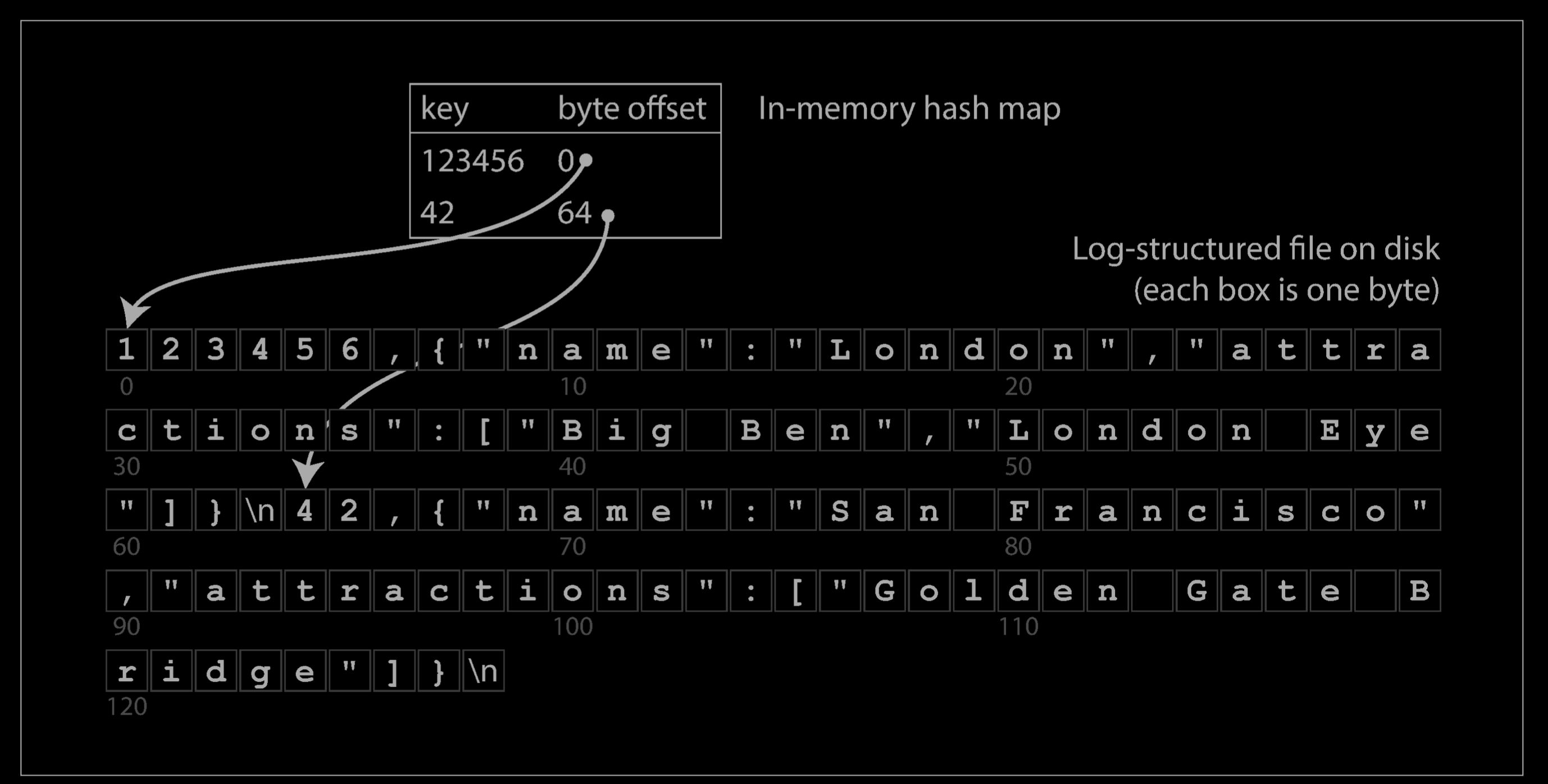
Let’s say our data storage consists only of appending to a file, as in the preceding example. Then the simplest possible indexing strategy is this: keep an in-memory hash map where every key is mapped to a byte offset in the data file—the location at which the value can be found, as illustrated below. Whenever you append a new key-value pair to the file, you also update the hash map to reflect the offset of the data you just wrote (this works both for inserting new keys and for updating existing keys). When you want to look up a value, use the hash map to find the offset in the data file, seek to that location, and read the value.
This may sound simplistic, but it is a viable approach. In fact, this is essentially what Bitcask (the default storage engine in Riak) does. Bitcask offers high-performance reads and writes, subject to the requirement that all the keys fit in the available RAM, since the hash map is kept completely in memory. The values can use more space than there is available memory, since they can be loaded from disk with just one disk seek. If that part of the data file is already in the filesystem cache, a read doesn’t require any disk I/O at all.
A storage engine like Bitcask is well suited to situations where the value for each key is updated frequently. For example, the key might be the URL of a cat video, and the value might be the number of times it has been played (incremented every time someone hits the play button). In this kind of workload, there are a lot of writes, but there are not too many distinct keys—you have a large number of writes per key, but it’s feasible to keep all keys in memory.
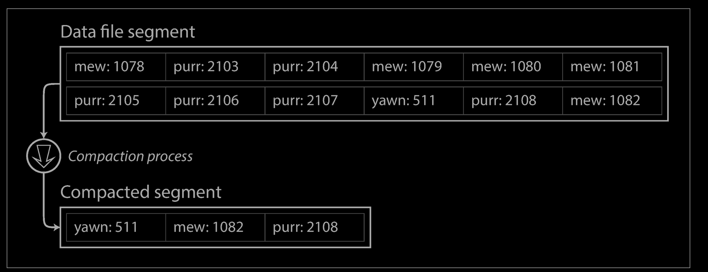
As described so far, we only ever append to a file—so how do we avoid eventually running out of disk space? A good solution is to break the log into segments of a certain size by closing a segment file when it reaches a certain size, and making subsequent writes to a new segment file. We can then perform compaction on these segments, as illustrated below Compaction means throwing away duplicate keys in the log, and keeping only the most recent update for each key.
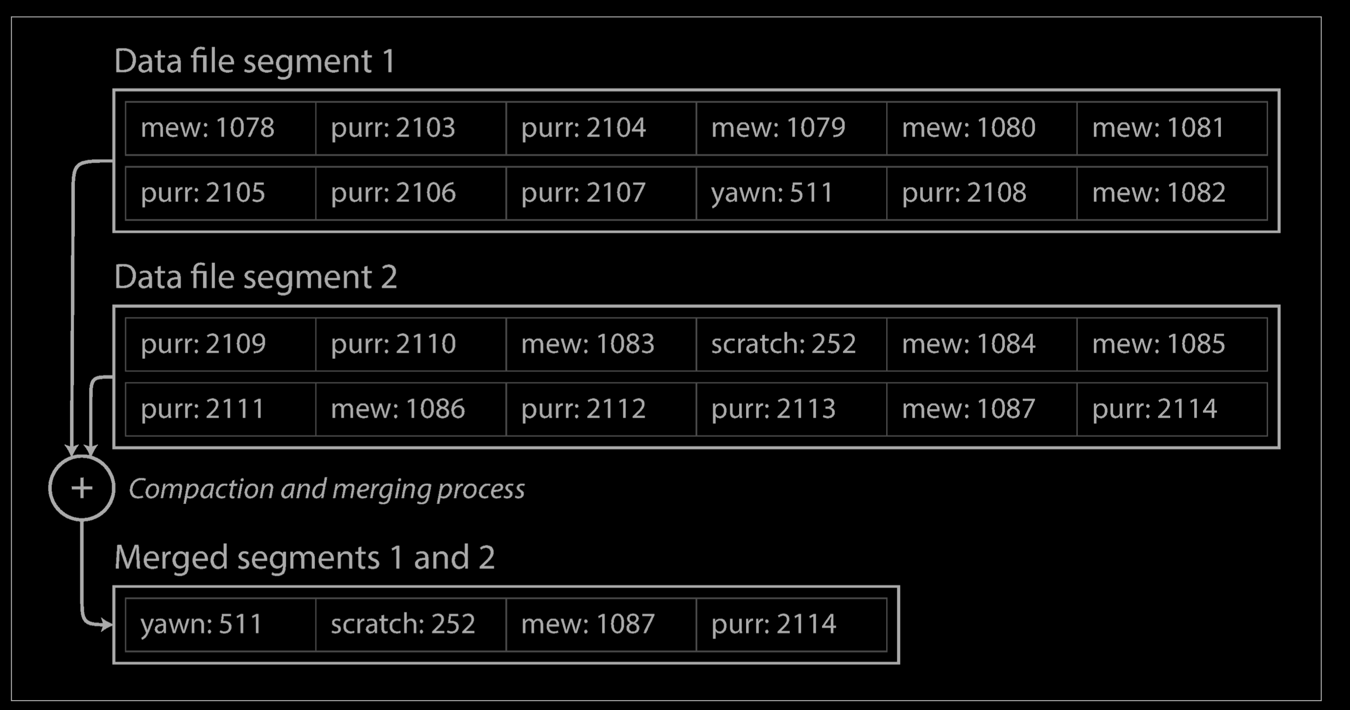
Moreover, since compaction often makes segments much smaller (assuming that a key is overwritten several times on average within one segment), we can also merge several segments together at the same time as performing the compaction, as shown below. Segments are never modified after they have been written, so the merged segment is written to a new file. The merging and compaction of frozen segments can be done in a background thread, and while it is going on, we can still continue to serve read and write requests as normal, using the old segment files. After the merging process is complete, we switch read requests to using the new merged segment instead of the old segments—and then the old segment files can simply be deleted.
Each segment now has its own in-memory hash table, mapping keys to file offsets. In order to find the value for a key, we first check the most recent segment’s hash map; if the key is not present we check the second-most-recent segment, and so on. The merging process keeps the number of segments small, so lookups don’t need to check many hash maps.
Lots of detail goes into making this simple idea work in practice. Briefly, some of the issues that are important in a real implementation are:
- File format: CSV is not the best format for a log. It’s faster and simpler to use a binary format that first encodes the length of a string in bytes, followed by the raw string (without need for escaping).
- Deleting records: If you want to delete a key and its associated value, you have to append a special deletion record to the data file (sometimes called a tombstone). When log segments are merged, the tombstone tells the merging process to discard any previous values for the deleted key.
- Crash recovery: If the database is restarted, the in-memory hash maps are lost. In principle, you can restore each segment’s hash map by reading the entire segment file from beginning to end and noting the offset of the most recent value for every key as you go along. However, that might take a long time if the segment files are large, which would make server restarts painful. Bitcask speeds up recovery by storing a snapshot of each segment’s hash map on disk, which can be loaded into memory more quickly.
- Partially written records: The database may crash at any time, including halfway through appending a record to the log. Bitcask files include checksums, allowing such corrupted parts of the log to be detected and ignored.
- Concurrency control: As writes are appended to the log in a strictly sequential order, a common implementation choice is to have only one writer thread. Data file segments are append-only and otherwise immutable, so they can be read concurrently by multiple threads.
An append-only log seems wasteful at first glance: why don’t you update the file in place, overwriting the old value with the new value? But an append-only design turns out to be good for several reasons:
- Appending and segment merging are sequential write operations, which are generally much faster than random writes, especially on magnetic spinning-disk hard drives. To some extent sequential writes are also preferable on flash-based solid state drives (SSDs).
- Concurrency and crash recovery are much simpler if segment files are appendonly or immutable. For example, you don’t have to worry about the case where a crash happened while a value was being overwritten, leaving you with a file containing part of the old and part of the new value spliced together.
- Merging old segments avoids the problem of data files getting fragmented over time.
However, the hash table index also has limitations:
- The hash table must fit in memory, so if you have a very large number of keys, you’re out of luck. In principle, you could maintain a hash map on disk, but unfortunately it is difficult to make an on-disk hash map perform well. It requires a lot of random access I/O, it is expensive to grow when it becomes full, and hash collisions require fiddly logic.
- Range queries are not efficient. For example, you cannot easily scan over all keys between kitty00000 and kitty99999—you’d have to look up each key individually in the hash maps.
In the next section we will look at an indexing structure that doesn’t have those limitations.
Background
During the 1990s, disk bandwidth, processor speed and main memory capacity were increasing at a rapid rate.
With increase in memory capacity, more items could now be cached in memory for reads. As a result, read workloads were mostly absorbed by the operating system page cache. However, disk seek times were still high due to the seek and rotational latency of physical R/W head in a spinning disk. A spinning disk needs to move to a given track and sector to write the data. In the case of random I/O, with frequent read and write operations, the movement of physical disk head becomes more than the time it takes to write the data. From the LFS paper, traditional file systems utilizing a spinning disk, spends only 5-10% of disk’s raw bandwidth whereas LFS permits about 65-75% in writing a new data (rest is for compaction). Traditional file systems write data at multiple places: the data block, recovery log and in-place updates to any metadata. The only bottleneck in file systems now, were during writes. As a result, there was a need to reduce writes and do less random I/O in file systems. LFS came with the idea that why not write everythng in a single log (even the metadata) and treat that as a single source of truth.
Log structured file systems treat your whole disk as a log. Data blocks are written to disk in an append only manner along with their metadata (inodes). Before appending them to disk, the writes are buffered in memory to reduce the overhead of disk seeks on every write. On reaching a certain size, they are then appended to disk as a segment (64kB-1MB). A segment contains data blocks containing changes to multitude of files along with their inodes. At the same time on every write, an inode map (imap) is also updated to point to the newly written inode number. The imap is also then appended to the log on every such write so it’s a just single seek away.
We’re not going too deep on LFS, but you get the idea. LSM Tree steals the idea of append only style updates in a log file and write buffering and has been adopted for use as a storage backend for a lot of write intensive key value database systems. Now that we know of their existence, let’s look at them more closely.
Log-structured merge-trees (LSM trees)
A log-structured merge-tree (LSM tree) is a data structure typically used when dealing with write-heavy workloads. The write path is optimized by only performing sequential writes.
- LSM trees are the core data structure behind many modern NoSQL Databases e.g. BigTable, Cassandra, HBase, RocksDB, and DynamoDB.
- LSM trees are used in data stores such as Apache AsterixDB, Bigtable, HBase, LevelDB, Apache Accumulo, SQLite4 Tarantool, RocksDB, WiredTiger, Apache Cassandra, InfluxDB and ScyllaDB.
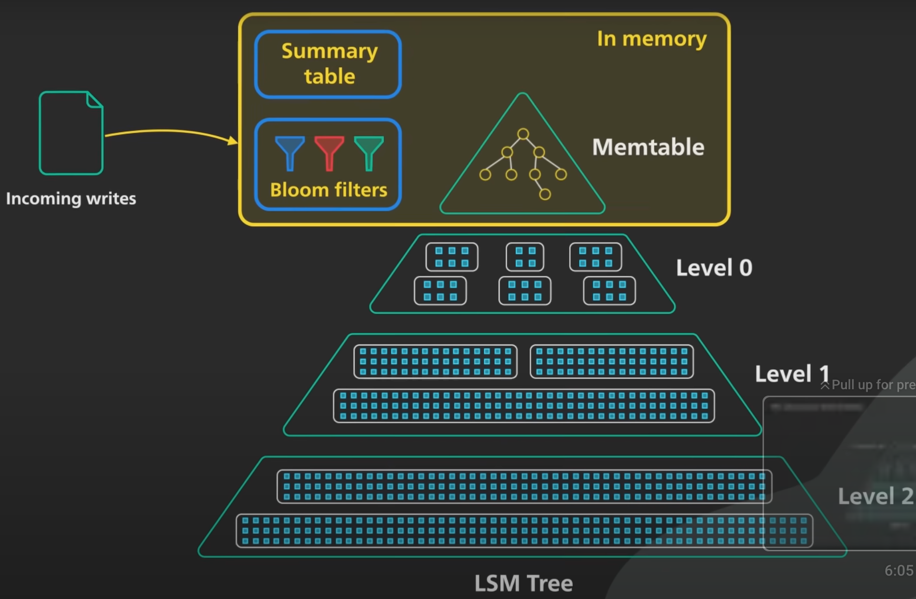
Like other search trees, an LSM-tree contains key-value pairs. It maintains data in two or more separate components (sometimes called SSTables).
The LSM Trees use two separate structures to store data and perform optimised Reads and Writes over them.
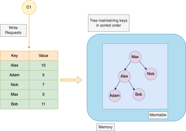
- The first structure is smaller and stored in the memory in the form of a Red Black Tree or an AVL Tree. This structure is also known as Memtable.
- The second structure is comparatively larger and is present on the Disk, It is stored in the form of SS Tables also known as Sorted String Tables.
As data files accumulate on disk, they are organized into levels based on their size and age. The lower levels contain larger and older files, while the higher levels contain smaller and newer files. The levels are merged periodically to maintain a compact and efficient data structure, with the smallest and newest data being prioritized to ensure fast access times.
Components
Memtables
The Memtables are maintained in the memory and every Database write is directed to this Memtable. These Memtables are generally an implementation of Tree data structure in order to maintain the keys in a sorted format. It can be a Red-Black Tree or an AVL Tree.
Sorted Strings Table (SSTable)
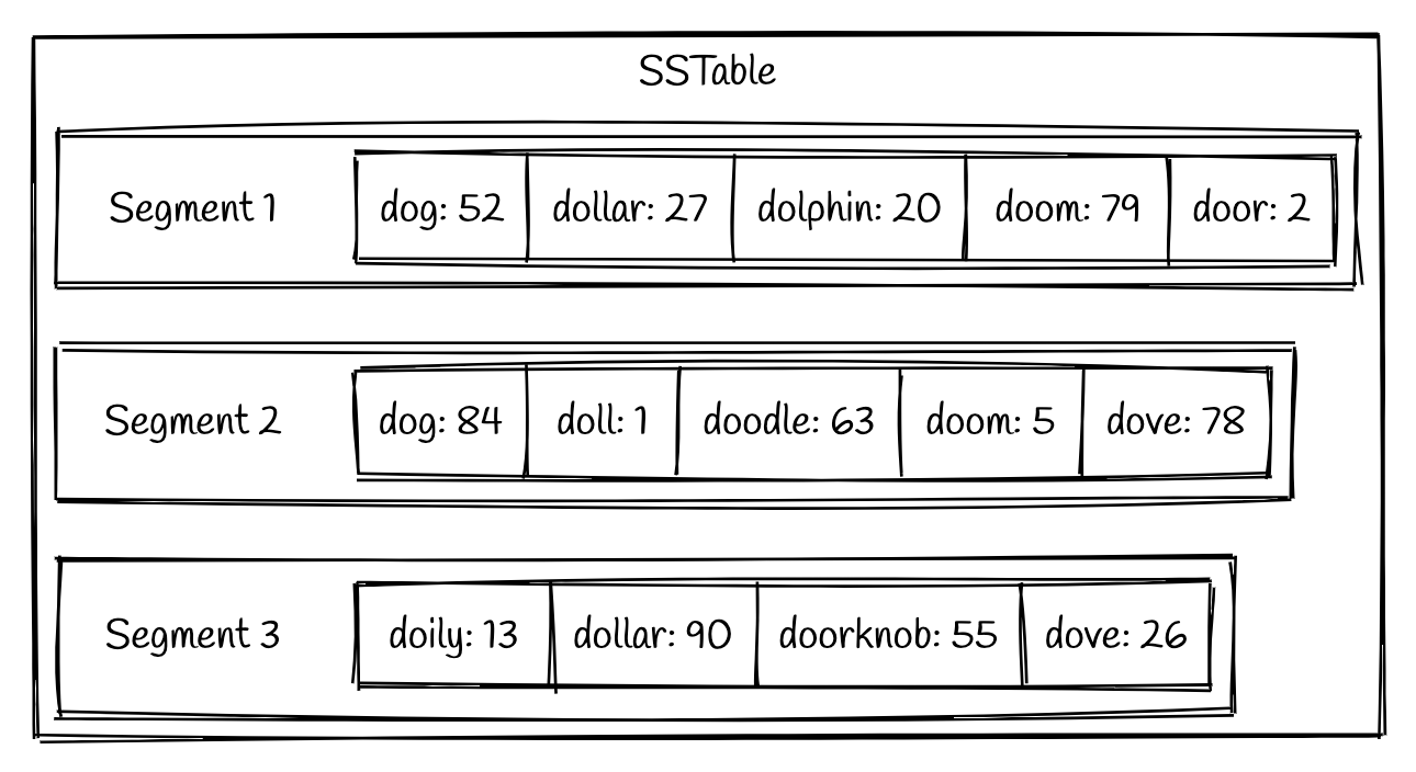
LSM trees are persisted to disk using a Sorted Strings Table (SSTable) format. As indicated by the name, SSTables are a format for storing key-value pairs in which the keys are in sorted order. Each key only appears once within each merged segment file (the compaction process already ensures that.
An SSTable will consist of multiple sorted files called segments.
A simple example could look like this:
Advantages
SSTables have several big advantages over log segments with hash indexes:
-
Merging segments is simple and efficient, even if the files are bigger than the available memory. The approach is like the one used in the mergesort algorithm and is illustrated below: you start reading the input files side by side, look at the first key in each file, copy the lowest key (according to the sort order) to the output file, and repeat. This produces a new merged segment file, also sorted by key.
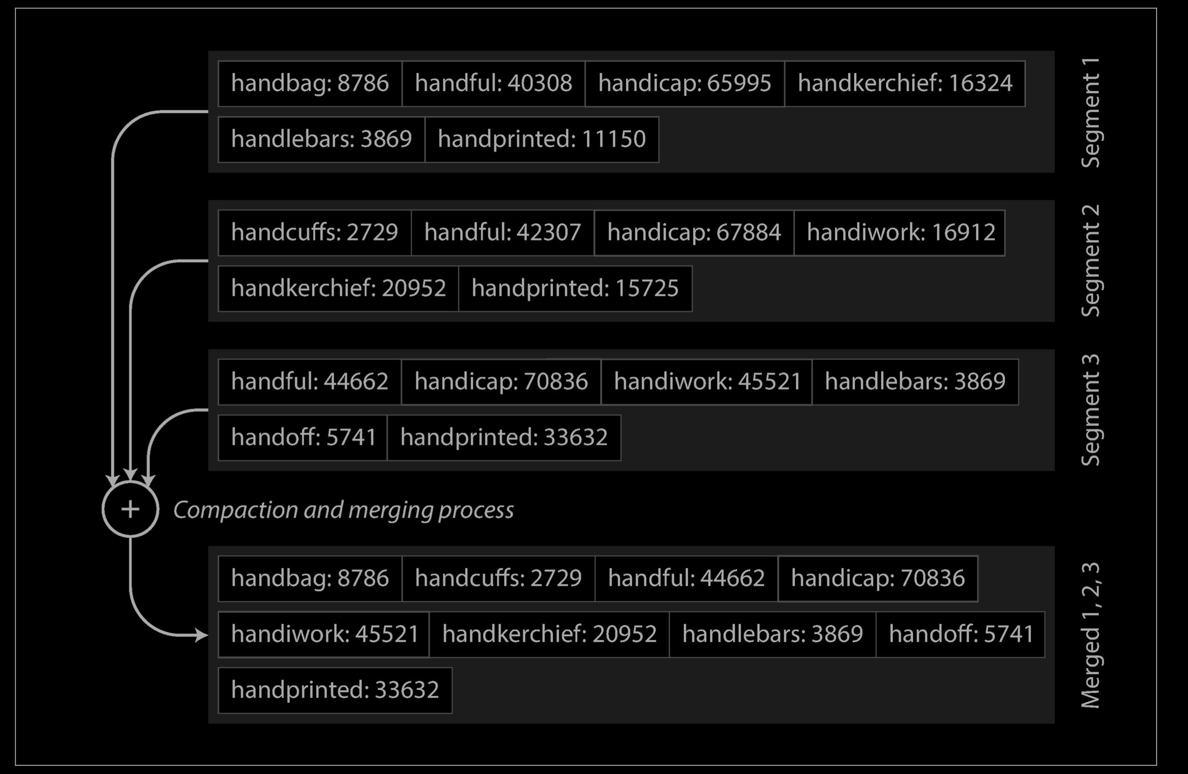
What if the same key appears in several input segments? Remember that each segment contains all the values written to the database during some period of time. This means that all the values in one input segment must be more recent than all the values in the other segment (assuming that we always merge adjacent segments). When multiple segments contain the same key, we can keep the value from the most recent segment and discard the values in older segments.
-
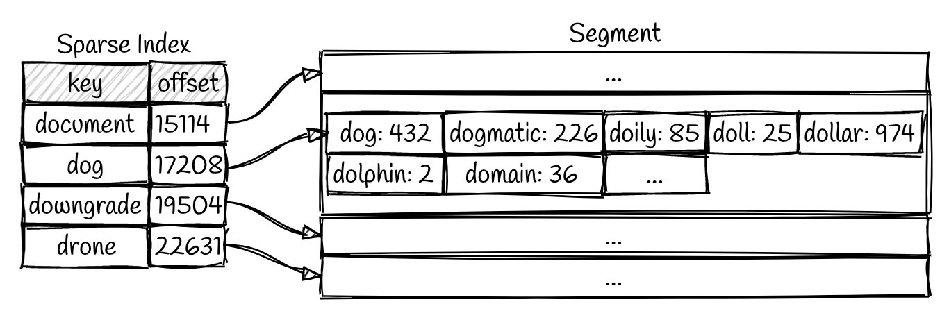
In order to find a particular key in the file, you no longer need to keep an index of all the keys in memory. See below for an example: say you’re looking for the key
handiwork, but you don’t know the exact offset of that key in the segment file. However, you do know the offsets for the keyshandbagandhandsome, and because of the sorting you know thathandiworkmust appear between those two. This means you can jump to the offset forhandbagand scan from there until you find handiwork (or not, if the key is not present in the file).You still need an in-memory index to tell you the offsets for some of the keys, but it can be sparse(稀疏的): one key for every few kilobytes of segment file is sufficient, because a few kilobytes can be scanned very quickly.
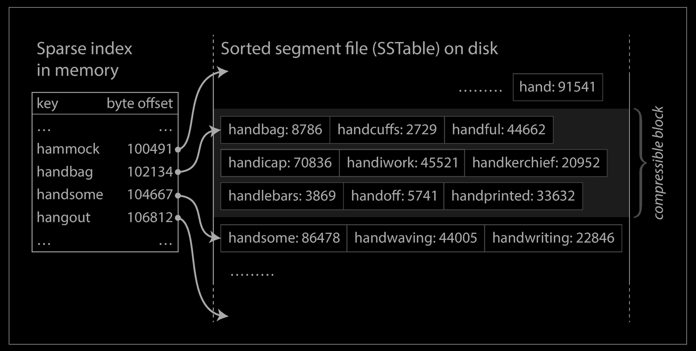
- Since read requests need to scan over several key-value pairs in the requested range anyway, it is possible to group those records into a block and compress it before writing it to disk (indicated by the shaded area above. Each entry of the sparse in-memory index then points at the start of a compressed block. Besides saving disk space, compression also reduces the I/O bandwidth use.
Operation
Writing
When a Write is issued to the Database it is simply written to the Memtable in the memory. Since the writes take place in the memory, the process is very fast.
Under the hood we have used a Tree Structure in order to store keys in a sorted format. Since the Tree structure used here is a Self Balancing tree, it guarantees the Writes and Reads to be performed within Logarithmic time.
We can use AVL Tree for this implementation which supports addition of nodes in logarithmic time and maintains them in a sorted order. They also allow reading all the nodes in a sorted format in linear time. This advantage of the AVL Tree will help us in future when we flush the data to the disk from the memory.
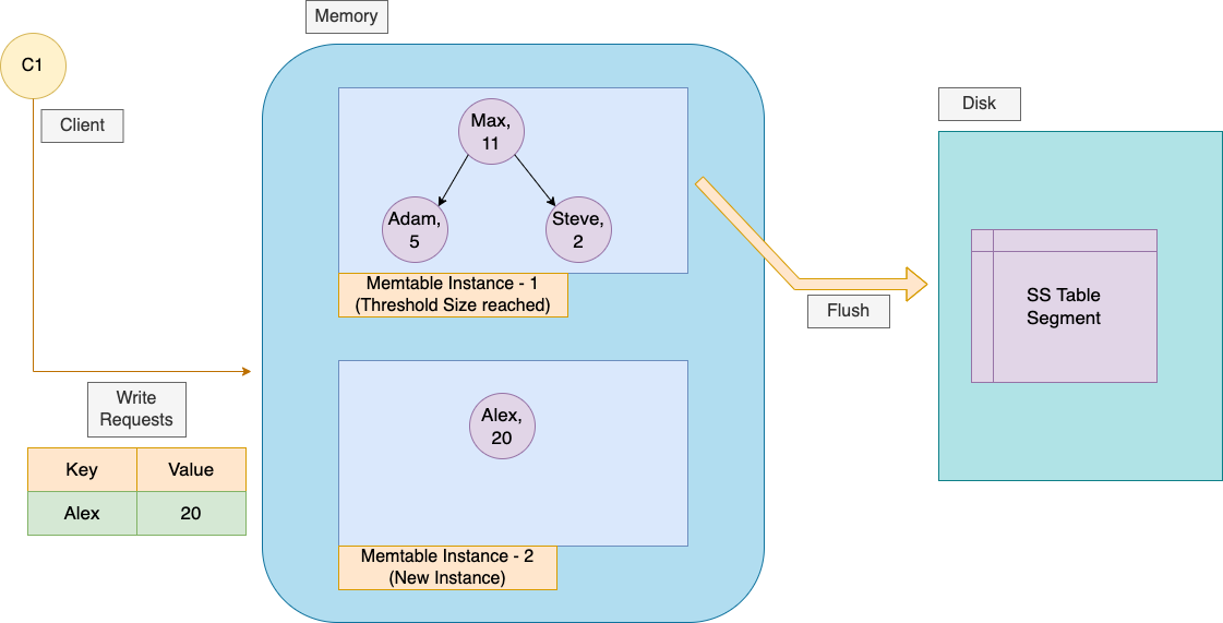
Our writes get stored in this AVL tree until the tree reaches a predefined size. Once the AVL tree has enough entries, it is flushed to disk as a new segment in the form of the SS Tables also known as Sorted String Tables on disk in sorted order. This can be done efficiently because the tree already maintains the key-value pairs sorted by key. The new SSTable file becomes the most recent segment of the database. While the SSTable is being written out to disk, writes can continue to a new memtable instance.
If the database crashes, the most recent writes (which are in the memtable but not yet written out to disk) are lost. In order to avoid that problem, we can keep a separate log on disk to which every write is immediately appended,. That log is not in sorted order, but that doesn’t matter, because its only purpose is to restore the memtable after a crash. Every time the memtable is written out to an SSTable, the corresponding log can be discarded.
The memtables are nothing but a self balancing tree data structure that maintains the keys in a sorted order. Hence it’s very easy to iterate over the keys in a sorted order. The keys are read in a sorted order from the memtable and are further stored on the Disk.
When the memtable gets bigger than some threshold—typically a few megabytes —write it out to disk as an SSTable file. This can be done efficiently because the tree already maintains the key-value pairs sorted by key. The new SSTable file becomes the most recent segment of the database. While the SSTable is being written out to disk, writes can continue to a new memtable instance.
Reading
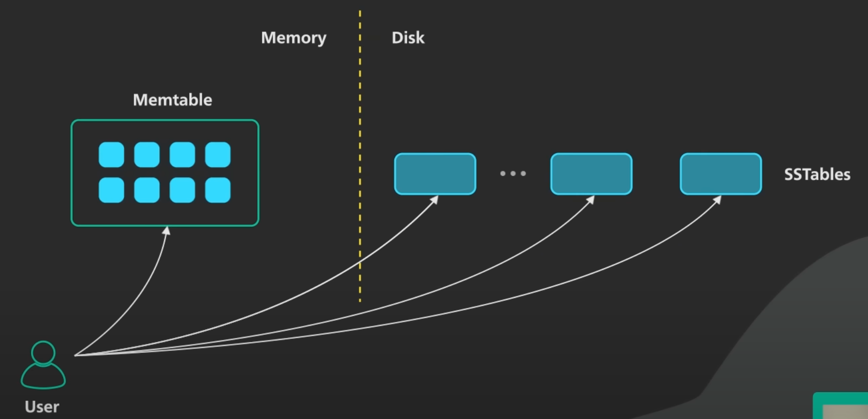
- In order to serve a read request, first try to find the Key in the Memtable (memory),
- Once the Key is not found in the Memtable then it is looked in the SS Table (on the disk), by the following order - the most recent on-disk segment, then in the next-older segment, etc.
- We are not required to look into every key inside the SS Table to read the value of the searched key. Instead we can maintain a sparse in-memory index table to optimise this. We can store some keys with their memory location in this table. Say for every 1000 key-value pair block, we can store the first key of that block along with its memory address in the in-memory sparse index table.
- We can use this index to quickly find the offsets for values that would come before and after the key we want. Now we only have to scan a small portion of each segment file based on those bounds. For example, let’s consider a scenario where we want to look up the key
dollarin the segment above. We can perform a binary search on our sparse index to find thatdollarcomes betweendoganddowngrade. Now we only need to scan from offset 17208 to 19504 in order to find the value (or determine it is missing). - This is a nice improvement, but what about looking up records that do not exist? We will still end up looping over all segment files and fail to find the key in each segment. This is something that a bloom filter can help us out with. A bloom filter is a space-efficient data structure that can tell us if a value is missing from our data. We can add entries to a bloom filter as they are written and check it at the beginning of reads in order to efficiently respond to requests for missing data.
- We can still ask why we are not using Binary Search to look for a key in the SS Table block, since it already maintains the entry sorted by keys. Generally the values do not have a fixed size and hence it is difficult to tell where one record ends and the next one starts. Hence we naively perform a Linear-Search over the block to look for our key.
Compaction(压实)
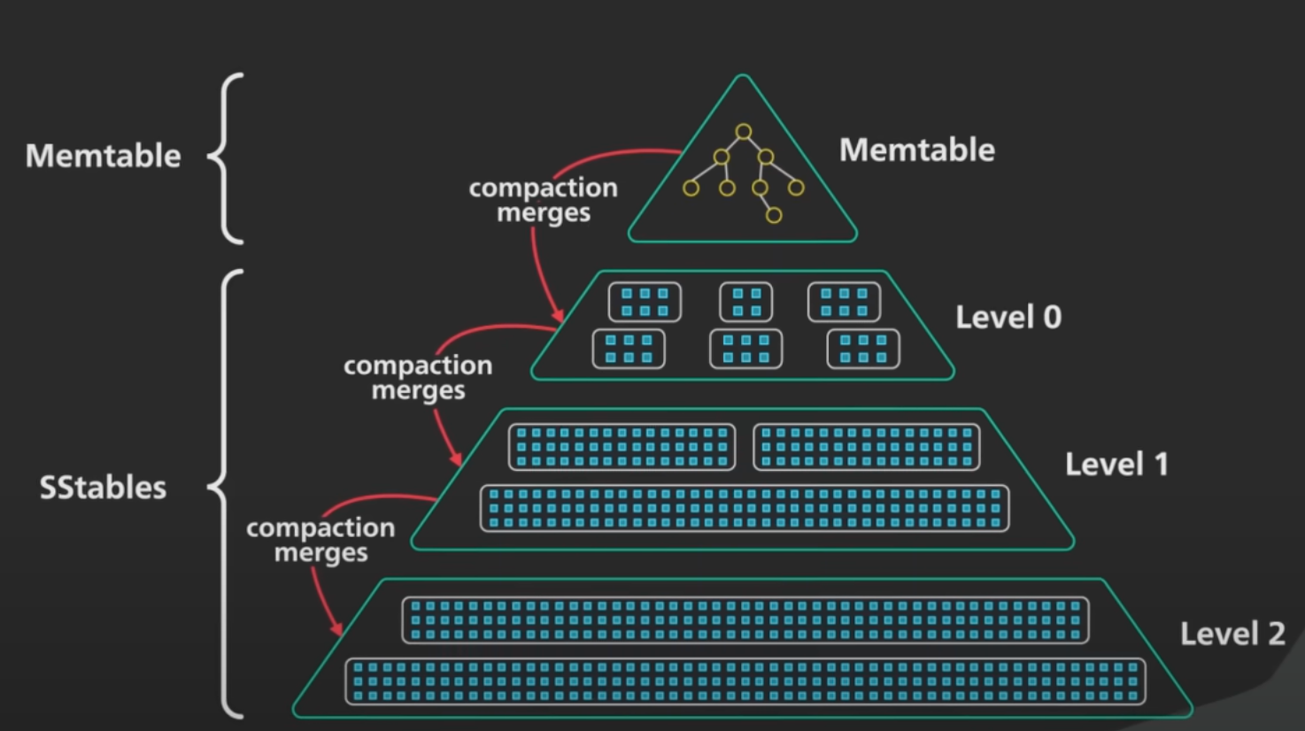
Over time, this system will accumulate more segment files as it continues to run. These segment files need to be cleaned up and maintained in order to prevent the number of segment files from getting out of hand. This is the responsibility of a process called compaction. Compaction is a background process that is continuously combining old segments together into newer segments.
Suppose we have three segments of SS Tables with us over the disk. The merging process will look similar to the process we follow in the Merge-Sort Algorithm to merge two sorted arrays. The idea is to keep a pointer at the start of each Table segment and pick the smallest key and add it to the resulting segment and move that pointer one step ahead. We keep iterating over this process until all the key value pairs in all segments are pushed to the resulting segment.
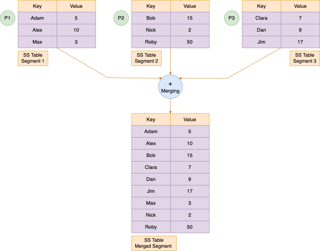
While Merging we also take care of the duplicate keys. If the same key appears in multiple segments then we keep the key from the most recent segment and discard the keys from the older segments. This process is known as Compaction.
Maintaining all the keys in a sorted order in every segment helps in the merging process. It helps generate a merged sorted-ordered segment in linear time. This is a big advantage over the Hash-based data structures.
Compaction Strategies
A compaction strategy must choose which files to compact, and when to compact them. There are a lot of different compaction strategies that impact the read/write performance and the space utilization in the LSM Tree. Some of the popular compaction strategies that are used in production systems are:
- Size-tiered compaction stratey (STCS)
- The idea behind STCS is to compact small
SSTables into mediumSSTables when the LSM-tree has enough smallSSTables and compact mediumSSTables into largeSSTables when LSM-tree has enough mediumSSTables. - This is write optimized compaction strategy and is the default one used in ScyllaDB and Cassandra. But it has high space amplification, so other compaction strategies such as leveled compaction were developed.
- The idea behind STCS is to compact small
- Leveled compaction strategy (LBCS)
- The idea of LBCS is to organize data into levels and each level contains one sorted run. Once a level accumulates enough data, some of the data at this level will be compacted to the higher level.
- Improves over size-tiered and reduces read amplification as well as space amplification. This is the default in LevelDB.
- Time windowed compaction strategy - Used for time series databases. In this strategy, a time window is used post which compaction is triggered.
The above are not the only strategies and various systems have developed their own such as the hybrid compaction strategy in ScyllaDB.
Deletion
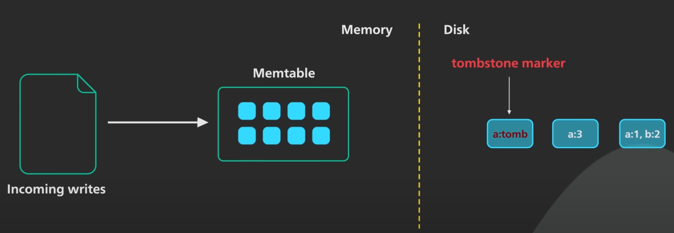
If you want to delete a key and its associated value, you have to append a special deletion record to the data file (sometimes called a tombstone). When log segments are merged, the tombstone tells the merging process to discard any previous values for the deleted key.
SSTable Enchancements
In practical implementations, SSTable files are also augmented with a SSTable summary and an index file which acts as a first point of contact when reading data from an SSTable. In this case, the SSTable is split into data files, an index file and a summary file (used in Casssandra and ScyllaDB).
SSTable data file
The SSTable data files are usually encoded in a specific format with any required metadata and the key value entries are stored in chunks called blocks. These blocks may also be compressed to save on disk space. Different levels may use different compression algorithms. They also employ checksums at each block to ensure data integrity.
SSTable index file
The index file lists the keys in the data file in order, giving for each key its position in the data file.
SSTable summary file
The SSTable summary file is held in memory and provides a sample of keys for fast lookup in the index file. Think of it like an index for the SSTable index file. To search for a specific key, the summary file is consulted first to find a short range of position in which the key can be found and the loads up that specific offset in memory.
Operations
Performance Optimizations
As always, a lot of detail goes into making a storage engine perform well in practice. For example, the LSM-tree algorithm can be slow when looking up keys that do not exist in the database: you have to check the memtable, then the segments all the way back to the oldest (possibly having to read from disk for each one) before you can be sure that the key does not exist. In order to optimize this kind of access, storage engines often use additional Bloom filters.
- A Bloom filter is a memory-efficient data structure for approximating the contents of a set. It can tell you if a key does not appear in the database, and thus saves many unnecessary disk reads for nonexistent keys.)
Drawbacks of LSM Trees
Any technology introduced, brings with it its own set of tradeoffs. LSM Tree is no different. The main disadvantage of LSM Tree is the cost of compaction which affects read and write performance. Compaction is the most resource intensive phase of LSM Tree due to compression/decompression of data, copying and comparision of keys involved in the process. A chosen compaction strategy must try to minimize read amplification, write amplification and space amplification. Another drawback of LSM Tree is the extra space required to perform compaction. This is certainly visible in size tiered compaction strategy and so other compaction strategies like leveled compaction are used. LSM Tree also makes reads slow in the worst case. Due to the append only nature, reads will have to search in SSTable at the lowest level. There’s file I/O involved in seeks which makes reads slow.
Despite their disadvantages, LSM Trees have been in use in quite a lot of database systems and has become the de-facto pluggable storage engine in lot of storage scenarios.
LSM Trees in the wild
LSM trees have been used in many NoSQL databases as their storage engine. They are also used as embedded databases and for any simple but robust data persistance uses cases such as search engine indexes.
One of the first projects to make use of LSM Trees was the Lucene search engine (1999). Google BigTable (2005), a distributed database also uses LSM Tree in their underlying tablet server design and is being used for holding petabytes of data for Google Crawl and analytics. It was then discovered by BigTable authors that the design of BigTable’s “tablet” (storage engine node) could be abstracted out and be used as a key value store.
Born off of that, came LevelDB (2011) by the same authors which uses LSM Tree as its underlying data structure. This gave rise to pluggable storage engines and embedded databases. Around the same time in 2007, Amazon came up with DynamoDB which uses the same underlying LSM Tree structure along with a masterless distributed database design.
Dynamo DB inspired the design of Cassandra (2008), which is an open source distributed NoSQL database. Cassandra inspired ScyllaDB (2015) and others. InfluxDB (2015), a time series database also uses LSM Tree based storage engine called Time structured merge tree.
Inspired from LevelDB, Facebook forked LevelDB and created RocksDB (2012), a more concurrent and efficient key value store that uses multi-threaded compaction to improve read and write performance. Recently Bytedance, the company behind TikTok has also released a key value store called terakdb that improves over RocksDB. Sled is another embedded key value store in Rust, that uses a hybrid architecture of B+ Trees and LSM Tree (Bw Trees). These fall under the category of embedded data stores.
Reference
- Designing Data Intensive Applications
- https://www.cs.umb.edu/~poneil/lsmtree.pdf
- https://en.wikipedia.org/wiki/Log-structured_merge-tree
- https://yetanotherdevblog.com/lsm/
- https://tikv.github.io/deep-dive-tikv/key-value-engine/B-Tree-vs-Log-Structured-Merge-Tree.html
- https://www.linkedin.com/pulse/data-structures-powering-our-database-part-2-saurav-prateek/
- http://www.benstopford.com/2015/02/14/log-structured-merge-trees/
- https://dev.to/creativcoder/what-is-a-lsm-tree-3d75
- https://lrita.github.io/images/posts/database/lsmtree-170129180333.pdf